


Chapter 5 Classical Feedback Analysis
© National Instruments Corporation 5-9 Xmath Control Design Module
Referring to the entire closed-loop system in Figure 5-1 as G
cl
, the poles of
G
cl
are the roots of its denominator—that is, the values of s such that either
of the following is true:
The magnitude (absolute value) of G(s) is 1 at each pole of G
cl
(s), and the
phase (given by the four-quadrant arctangent) of G(s) is –180° at each pole
of G
cl
(s). For any neutrally stable system, the frequency response
magnitude will be equal to 1 (or 0 dB) and the phase will be –180° at the
frequency at which the closed-loop roots fall on the imaginary axis.
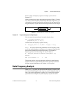
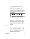
This analysis is often applied to systems where G(s) consists of a gain, K,
and a dynamic model, H(s), in series (as shown in Figure 5-1). For cases
in which increasing the gain leads to system instability, the system will be
stable for a given value of K if the magnitude of KH(s) is less than 1 at any
frequency at which the phase of KH(s) is 180° [FPE87]. You can measure
how close a system is to instability by examining the value of the magnitude
and phase at these critical values. These measures are termed the gain
margin and the phase margin. These are important because real-life models
are prone to uncertainties and changes in gain or phase. Typically, systems
become unstable with gains that are too high or have too much phase lag.
Refer to Example 5-4.
The gain margin indicates by how much the gain can be raised before the
closed-loop system becomes unstable. This critical gain value at which
instability results can be thought of in several ways. As described
previously, this gain value results in the closed-loop poles of the system
being located on the imaginary axis. In terms of the Nyquist stability
criterion, discussed in more detail under
nyquist( ), this is the gain value
at which the Nyquist plot crosses the negative real axis, where the phase is
–180 degrees. The gain margin itself is the reciprocal of this value,
expressed in decibels.
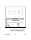
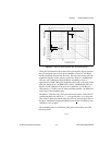
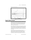
The Bode plot provides a clear visual interpretation of the gain margin as
the number of decibels by which the gain exceeds zero when the phase
equals –180 degrees. The phase margin is the difference between the phase
at the point where the response crosses the unit circle (has unit magnitude,
or a gain of 0 decibels) and –180 degrees. These margins provide a measure
of how near the closed-loop system roots are to instability. Depending on
the complexity of the system, there may be multiple gain and/or phase
margins.
1 Gs() 0=+
Gs() 1–=