


Chapter 2 Linear System Representation
© National Instruments Corporation 2-3 Xmath Control Design Module
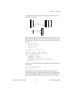
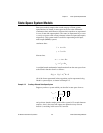
form the same transfer function as that derived in the preceding transfer
function equation using known pole, zero, and gain values:
(2-4)
The systems represented in Equations 2-3 and 2-4 can be represented using
Xmath’s system objects, as shown in Example 2-1.
The Xmath transfer function system object currently can be used to
represent single-input, single-output systems only. State-space form can
be used to describe systems with multiple inputs or outputs. For more
information, refer to the State-Space System Models section.
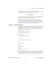
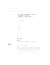
Example 2-1 Creating Transfer Functions
The polynomials in the numerator and denominator of the transfer function
in Equation 2-3 are both in coefficients form, (described using just
coefficients, not roots).
makepoly( ) creates two polynomials and passes
them to the
system( ) function:
num3 = makepoly([2,-1],"s");
den3 = makepoly([1,6,8],"s");
H3 = system(num3,den3)
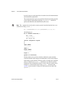
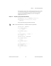
This displays as:
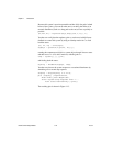
H3 (a transfer function) =
2s - 1
----------
s
2
+ 6s + 8
initial integrator outputs
0
0
Input Names
-----------
Input 1
Output Names
------------
Output 1
System is continuous
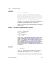
The three statements used to create the transfer function could be more
compactly combined as one. The use of s as the variable in which to express
the transfer function is optional. Any variable, including the default x, can
Hs()
2 s 0.5–()
s 2+()s 4+()
---------------------------------=