Chapter 4 System Analysis
© National Instruments Corporation 4-5 Xmath Control Design Module
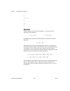
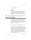
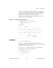
ans (a column vector) =
-0.98875 + 2.4773 j
-0.98875 - 2.4773 j
k (a scalar) = 1.34P
Algorithm
The algorithm used for state-space zero computation creates a
reduced-order S(λ), using Householder reflections to do the necessary
orthogonal row and column compressions of the state-space matrices.
The eigenvalues of this reduced matrix are then found using QZ. This
method handles the degenerate case and systems with zeros at infinity
[EmV82].
Note zeros( ) also can be used as a matrix building function when used with scalar or
matrix input. For more details on this usage, refer to the MATRIXx Help.
Partial Fraction Expansion
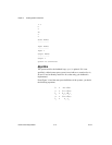
By inverse Laplace or z-transforming a transfer function, you can identify
the impulse response based on knowledge of the system pole and zero
locations. The most convenient form to use in doing this is the partial
fraction expansion of the transfer function. Each term of the partial fraction
expansion has a constant numerator—the residue—and a pole term
denominator, as shown in the following equation, where p
2
is a repeated
pole, and p
4
and p
5
are a conjugate pair:
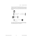
Each p
k
represents a pole of the system, and the corresponding r
k
is the
residue at that pole. If p
k
is a repeated pole, it has M residues, where M is
the multiplicity of the pole. Complex pole pairs have complex residue pairs.
If the transfer function contains a constant (or feedthrough) term, this term
is represented by the scalar value C in the preceding equation. The values
of the residues give the magnitude of the response from the inverse
transform of the respective partial fraction terms. For an example of
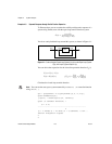
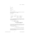
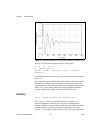
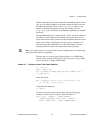
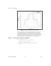
dynamic response with partial fraction expansion, refer to Example 4-3.
[Oga70] provides a good reference on partial-fraction expansion for
different orders of complex and real poles. [ChB84] contains a thorough
mathematical treatment of residues.
Hq() C
r
1
qp
1
+
--------------
r
2
qp
2
+()
2
---------------------
r
3
qp
3
+
--------------
α
4
q α
5
+
qp
4
+()qp
5
+()
--------------------------------------- …
r
n
qp
n
+
--------------++ ++ ++=


