Chapter 6 State-Space Design
© National Instruments Corporation 6-5 Xmath Control Design Module
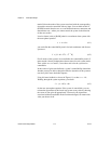
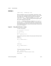
Beginning with the basic state-space equations (the Du output term can be
omitted without loss of generality):
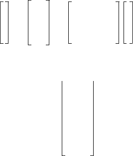
you can obtain expressions for the successive derivatives of the output term,
thus forming a complete description of the initial condition on the output:
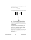
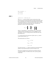
Generally, you term the following matrix
the observability matrix. If the rank of O is equal to n (where A is an n × n
matrix), you can always find a state vector which will realize the initial
conditions you want on the output, presuming that you know the initial
conditions on the input. If, however, the observability matrix loses rank
(is singular, in the SISO case), you will not be able to find states that give
you particular output conditions if those conditions lie in the null space of
the observability matrix.
The observability of a system is of particular importance when you want
to determine the actual values of the states based on our knowledge of the
system dynamics and the input and output values at a given time. If a system
is observable, you can create an observer, or estimator, to “guess” the
values of the states and use the information available to zero the state
estimate error as quickly and accurately as possible.
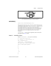
Referring to Figure 6-2 and tracing through the system equations, you can
obtain the time-update equation for the state estimate error
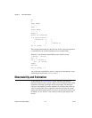
Figure 6-2 is a general observer block diagram where the output estimate
error is defined as
x
·
Ax Bu+=
yCx=
y
y
·
y
··
C
CA
CA
2
x
000
CB 00
CAB CB 0
u
u
·
u
··
+=
O
C
CA
CA
2
…
CA
n 1–
=
...
x
˜
xx
ˆ
.–=
y
˜
y
˜
yy
ˆ
.–=


