


183
Complex Samples General Linear Model
The parameter estimates are useful for quantifying the effect of each model term, but the estimated
marginal means tables can make it easier to interpret the model results.
Estimated Marginal Means
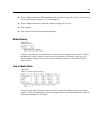
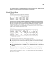
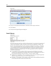
Figure 19-9
Estimated m arginal means by levels of Who shopping for
This table displays the model-estimated marginal means and standard errors of Amount spent at
the factor levels of Who shopping for. This table is useful for exploring the differences between
the levels of this factor. In this example, a customer who shops for him- or herself is expected
to spend about $308.53, while a customer with a spouse is expected to spend $370.34, and a
customer with dependents will spend $459.44. To see whether this represents a real difference or
is due to chance variation, look at the test results.
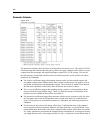
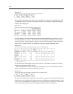
Figure 19-10
Individual test results for estimated marginal means of gender
The individual tests table displays two simple contrasts in spending.
The contrast e stimate is the difference in spending for the listed levels of Who shopping for.
The hypothesized value of 0.00 represents the belief that there is no difference in spending.
The Wald F statistic, with the displayed degrees of freedom, is used to test whether the
difference between a contrast estimate and hypothesized value is due to chance variation.
Since the significance values are less than 0.05, you can conclude that there are differences in
spending.
The values of the contrast estimates are different from the parameter estimates. This is because
there is an interaction term containing the Who shopping for effect. As a result, the parameter
estimate for shopfor=1 is a simple contrast between the levels Self and Self and Family at the
level From both of the variable Use coupons. The contrast estimate in this t able is averaged over
the levels of Use coupons.