


© 1997, 2004, 2006 TEXAS INSTRUMENTS INCORPORATED GETTING STARTED WITH THE CBR 2™ SONIC MOTION DETECTOR 33
Teacher Information
(cont.)
CBR 2™ motion detector plots—connecting the physical world and mathematics
The plots created from the data collected by EasyData or RANGER are a visual representation
of the relationships between the physical and mathematical descriptions of motion. Students
should be encouraged to recognize, analyze, and discuss the shape of the plot in both
physical and mathematical terms. Additional dialog and discoveries are possible when
functions are entered in the Y= editor and displayed with the data plots.
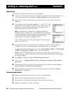
Performing the same calculations as
CBR 2™ motion detector is an interesting classroom
activity.
1. Collect sample data. Exit the EasyData application or RANGER program.
2. Use the sample times in
L1 in conjunction with the distance data in L2 to calculate the
velocity of the object at each sample time. Then compare the results to the velocity data
in
L3.
(
L2
n+1
+ L2
n
)à2 N (L2
n
+ L2
n-1
)à2
L3
n
=
L1
n+1
N L1
n
3. Use the velocity data in
L3 (or the student-calculated values) in conjunction with the
sample times in
L1 to calculate the acceleration of the object at each sample time. Then
compare the results to the acceleration data in
L4.
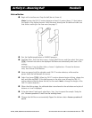
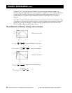
0 A Distance-Time plot represents the approximate position of an object (distance from the
CBR 2™ motion detector) at each instant in time when a sample is collected. y-axis units
are meters or feet; x-axis units are seconds.
0 A Velocity-Time plot represents the approximate speed of an object (relative to, and in
the direction of, the
CBR 2™ motion detector) at each sample time. y-axis units are
metersàsecond or feetàsecond; x-axis units are seconds.
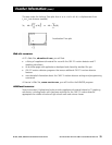
0 An Acceleration-Time plot represents the approximate rate of change in speed of an
object (relative to, and in the direction of, the
CBR 2™ motion detector) at each sample
time. y-axis units are metersàsecond
2
or feetàsecond
2
; x-axis units are seconds.
0 The first derivative (instantaneous slope) at any point on the Distance-Time plot is the
speed at that instant.
0 The first derivative (instantaneous slope) at any point on the Velocity-Time plot is the
acceleration at that instant. This is also the second derivative at any point on the
Distance-Time plot.
0 A definite integral (area between the plot and the x-axis between any two points) on the
Velocity-Time plot equals the displacement (net distance traveled) by the object during
that time interval.
0 Speed and velocity are often used interchangeably. They are different, though related,
properties. Speed is a scalar quantity; it has magnitude but no specified direction, as in
“6 feet per second.” Velocity is a vector quantity; it has a specified direction as well as
magnitude, as in “6 feet per second due North.”